The Interpolation Methods Available

The Interpolation Methods Available
In the applet, there are 7 interpolation methods implemented in this applet. Each method can be chosen from the top pull down menu after entering data points.

The following options are in this menu:
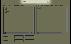
The Input page is used to enter data points and a range and domain for the graphs that are displayed.
You can enter functions in the box on the right. These functions will be displayed in many of the other parts of the applet. This is useful to compare a function with one of the interpolations that the applet will produce. This is where you enter the basis functions for the least squares method
When you enter points in the input page, the points are sorted by x value before being used by the interpolation methods. Thus the first basis function corresponds to the point with the smallest x value, not the point listed first.
This page will plot the points and graph the functions entered in the input page.
Lagrange Polynomial Interpolation
This page shows the basis functions in the four little graphs, and combined in the first large graph. The second graph shows the interpolating polynomial.
Newton Polynomial Interpolation
This page shows the basis functions in the four little graphs, and combined in the first large graph. The second graph shows the interpolating polynomial.
The first basis function is a constant function that goes through the first point. The second basis function is be a first degree polynomial that goes through the first 2 points. The third basis function is a second degree polynomial that goes through the first 3 points. etc.
Note the effects that moving a point has on the basis functions.
A linear spline is a simple piece-wise function that connects all the points with line segments. Each segment of the function is a line segment. The parts to the far left and far right, are just the horizontal line segments connecting to the first and last points.
The nth basis function is zero at all the points except for the nth point, at which the function is equal to 1. This is easily seen in the top four graphs. These basis functions are sometimes referred to as "hat functions." A linear combination of these basis functions can be seen in the lower right graph.
Also note that that for the first and last basis function, their far left or far right segment is equal to 1. There probably are a few other ways of creating linear splines with different types of extremities, but this is the method chosen for this applet.
This spline is the same as the linear spline, except that it uses 3rd degree curves instead of 1st degree line segments for each part of our piece-wise function.
This method is not necessarily an interpolation method. It can be used to find a closest fit curve to a set of data points.
For an example, paste this set of points into the applet's input section.
1.032258064516129,1.967741935483871
-1.4193548387096775,-0.7419354838709677
4.0,4.0
3.161290322580645,3.290322580645161
2.4838709677419355,2.5161290322580645
3.3870967741935485,2.903225806451613
1.8709677419354838,2.7096774193548385
0.29032258064516125,1.7741935483870968
-0.6129032258064516,0.0
-2.4516129032258065,-0.9354838709677419
-2.935483870967742,-2.3548387096774195
-3.4838709677419355,-1.4516129032258065
To try to do a closest fit line to these points, enter the two basis function of "1" and "x" in the functions part of the input page. As you probably know, all lines can be written in the form y=ax+b. Notice ax+b is a linear combination of x and 1. That is, we have something(a) times x plus something(b) times 1. You might also try using "2" instead of 1 for the basis function. This will not change the result.
Look at the graphs for this method, and you should see a line that is close to all the points.
You can also do a closest fit 3rd degree curve by using the basis function of "1", "x", "x^2", and "x^3".
If you want to find a curve in the form of y=a*sin(x) + b*x + c, you can use the basis functions of "sin(x)", "x", and "1". Try this with the data points listed above.
This is a method for fitting a curve to cyclical data. This could be used to find a curve that fits the yearly temperature, the amount of ozone in the air each day, or the number of people out on the beach during each day of the month. For these examples, the values should rise and drop and rise and drop continually, in a general pattern.
Try using these points as an example. You will see that the points represent one period of the data. The final point, will always stick to the same y value as the first point. That is why it might not move as you expect.
Here are two examples of data sets:
1.0,1.0
2.0,2.5
3.0,1.0
-2.967741935483871,0.9354838709677419
-2.129032258064516,-0.03225806451612903
-1.129032258064516,-0.9354838709677419
0.0,0.03225806451612903
1.0,0.9354838709677419
This method is highly prone to numerical error, and this can be easily seen with its sometimes erratic results. Internally for certain situations, the applet is having to solve a near singular matrix equation which is introducing significant errors into the calculations.
This fractal interpolation method is perhaps the most interesting of all the methods.
Try using these points as an example:
-2.967741935483871,0.0
-2.258064516129032,1.6774193548387095
-1.096774193548387,1.935483870967742
0.4838709677419355,0.0
These will give a nice picture of the fractal interpolation. If you use to many points, the applet will not draw the entire picture correctly, as the number of points plotted grows exponentially with the number of input points.
Notice with this example that the section in-between the two middle points is very similar to the overall shape of the entire fractal. This is also true of the other two sections, except that they are more stretched to fit between their two closest points.
Notice the basis functions are also fractal interpolations of each point with the y value changed either to "0" or "1". You might notice that the red points displayed are not really the points you entered.
©2002-2003 Isaac Dooley